Jupyter notebook is one of the packages under Project Jupyter, which started as a spin-off project from IPython. IPython is an enhanced interactive Python interpreter, developed by Fernando Perez in 2001. IPython notebook, a web-based interface was introduced in 2011.

It was later renamed as Jupyter notebook by adding programming environments (kernels) of Julia and R languages. (Jupyter is an acronym for JUlia, PYThon, and R). Now it supports many more languages such as Matlab, Scala, etc.

If you are using Anaconda distribution of Python, Jupyter notebook is already included in it. To install it individually in standard Python distribution, use a pip installer.

pip3 install jupyter

This will install the entire Jupyter system including notebook, QtConsole, and IPython kernel. It is also possible to install a notebook only.

pip3 install notebook

After installation check the version of the installation

C:\python37>jupyter --version

jupyter core     : 4.6.1

jupyter-notebook : 6.0.2

qtconsole        : 4.6.0

ipython          : 7.11.1

ipykernel        : 5.1.3

jupyter client   : 5.3.4

jupyter lab      : not installed

nbconvert        : 5.6.1

ipywidgets       : 7.5.1

nbformat         : 5.0.3

traitlets        : 4.3.3

To invoke notebook application, run the following command from a command prompt or Anaconda prompt. The command shell shows the following log:

C:\python37>jupyter notebook

[I 20:01:44.716 NotebookApp] Serving notebooks from local directory: C:\python37

[I 20:01:44.717 NotebookApp] The Jupyter Notebook is running at:

[I 20:01:44.720 NotebookApp] http://localhost:8888/?token=4f5bace23cb3ddbe24b650084d217f18cc58237c6ea8d02e

[I 20:01:44.720 NotebookApp]  or http://127.0.0.1:8888/?token=4f5bace23cb3ddbe24b650084d217f18cc58237c6ea8d02e

[I 20:01:44.721 NotebookApp] Use Control-C to stop this server and shut down all kernels (twice to skip confirmation).

[C 20:01:45.027 NotebookApp]

Jupyter notebook is a client-server application. The above command starts the notebook server at port 8888 (default) of localhost. Its client interface can be opened by visiting the URL (as shown in the command shell) with a browser.

To open a blank notebook, choose Python 3 kernel from the drop-down menu under the New button.

A blank notebook is opened in a new tab of the browser.

The notebook opens with a blank input cell. It acts as a traditional Python prompt (>>>) so that one or more valid Python statements can be entered into it. To execute Python code in the cell, use the Run from Cell menu or use the Ctrl+Enter shortcut.

A list of various shortcut combinations is available. They can be accessed from the Help menu and can be suitably edited as per convenience.

There are three types of cells in the Jupyter notebook. Code cells, Markdown cells, and Raw cells.

• Code cells: Jupyter notebook is primarily an enhanced and interactive REPL (READ, EVALUATE, PRINT, and LOOP) environment. The cell in which Python (or the kernel in use) code is entered is the input code cell. When it is run, the output is displayed in the output cell immediately below. The output cell displays the result in the form of text, or image (graphical output of code involving plotting libraries like Matplotlib), or HTML tables.
• Raw cells: These cells are not executed by the notebook server. Their contents are not rendered any differently from what they have when they are run. If a raw cell contains LaTex, it will be rendered when nbconvert operation is performed.
• Markdown cells: One of the most attractive features of the Jupyter notebook is that, along with the code, it can be interspersed with very neatly formatted documentation consisting of text with effects such as the bold or italic face, changing font color and size, numbered or bulleted list, tabular representation, images as well as hyperlinks. This type of content is entered in the Markdown cell. While this cell is not run or executed by the interpreter, it serves much more purpose than a comment. The contents of this type of cell are formatted with the help of markdown language syntax.

The following figure shows a notebook cell with markdown formatting and its rendered version when run.

To know more about formatting markdown in Jupyter, visit https://guides.github.com/features/mastering-markdown/

Magic commands

In addition to regular Python syntax, some special notebook commands can be entered in a notebook cell. These are called magic commands. These commands are prefixed with % symbol. To obtain a list of magic commands available, use %lsmagic command.

Commands starting with % are called line magics, while those starting with %% are called cell magics. The %ddir command implements the DOS Dir command.

In order to render HTML output in code cell, use %%html command

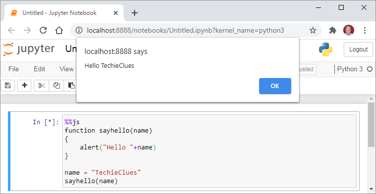
It also possible to embed a JavaScript code in a notebook with %%js cell magic command

The %matplotlib is an important magic command. Notebook app is capable of rendering Matplotlib graphs along with the code. By adding %matplotlib notebook command, the plots are interactively rendered. It means, if the associated data is altered, the plot changes dynamically without having to re-run the code cell.

A notebook in the client browser’s window can be saved with the .ipynb extension. It can be converted into distributable formats such as PDF, HTML, MD, or LaTeX. You can also generate a slide show out of notebook cells.

Jupyter notebook is extremely popular with data scientists for its interactive computing capabilities, production-ready output, and support to multiple data representation formats.